I am looking for some help automating the image resolution measurement. I am focusing on the sharp edge method. I would like to measure the resolution using python or a macro in ImageJ.
I have done many resolution measurements but I see a wide variation in the measurement, looking for a more repeatable method.
Do you have a test image you could post?
There are a few images in the discussion of resolution methods
I can also offer many raw images. For the methods I typically converted the color images to grayscale.


Thanks, let me know if this looks right:
# pip3 install scikit-image numpy matplotlib
import numpy as np
import matplotlib.pyplot as plt
from skimage import io, feature
from skimage.transform import probabilistic_hough_line
from scipy.ndimage import gaussian_filter1d

# ---------------------
# PART 1: LOGIC
# ---------------------

def load_image(path):
    return io.imread(path, as_gray=True)

def detect_edge_line(image):
    edges = feature.canny(image, sigma=2)
    lines = probabilistic_hough_line(edges, threshold=10, line_length=50, line_gap=10)
    if not lines:
        raise ValueError("No edge line detected.")
    longest_line = max(lines, key=lambda l: np.linalg.norm(np.subtract(l[0], l[1])))
    return longest_line

def get_perpendicular_lines(line, num_samples=3, length=50):
    (x1, y1), (x2, y2) = line
    dx, dy = x2 - x1, y2 - y1
    normal = np.array([-dy, dx], dtype=np.float64)
    normal /= np.linalg.norm(normal)
    sample_points_x = np.linspace(x1, x2, num_samples + 2)[1:-1]
    sample_points_y = np.linspace(y1, y2, num_samples + 2)[1:-1]
    perp_lines = []
    half_len = length / 2
    for mx, my in zip(sample_points_x, sample_points_y):
        start = (int(mx - normal[0] * half_len), int(my - normal[1] * half_len))
        end = (int(mx + normal[0] * half_len), int(my + normal[1] * half_len))
        perp_lines.append((start, end))
    return perp_lines

def extract_profile(image, line):
    (x0, y0), (x1, y1) = line
    length = int(np.hypot(x1 - x0, y1 - y0))
    x_vals = np.linspace(x0, x1, length)
    y_vals = np.linspace(y0, y1, length)
    profile = image[y_vals.astype(int), x_vals.astype(int)]
    return profile

def compute_lsf(esf):
    if np.mean(esf[:5]) > np.mean(esf[-5:]):
        esf = esf[::-1]  # flip so it's always increasing
    lsf = np.gradient(esf)
    return gaussian_filter1d(lsf, sigma=1.0)

def compute_fwhm(lsf):
    peak = np.max(lsf)
    half_max = peak / 2
    indices = np.where(lsf >= half_max)[0]
    return indices[-1] - indices[0] if len(indices) > 1 else None

# ---------------------
# PART 2: VISUALIZATION
# ---------------------

def visualize_results(image, edge_line, perp_lines, profiles, lsfs, fwhms):
    fig, axs = plt.subplots(2, 2, figsize=(12, 10))

    # Image + lines
    axs[0, 0].imshow(image, cmap='gray')
    axs[0, 0].set_title("Detected Edge and Sampled Lines")
    axs[0, 0].plot([edge_line[0][0], edge_line[1][0]],
                   [edge_line[0][1], edge_line[1][1]], 'r-', linewidth=2, label='Edge')
    for idx, line in enumerate(perp_lines):
        axs[0, 0].plot([line[0][0], line[1][0]],
                       [line[0][1], line[1][1]], '--', linewidth=1.5, label=f'Perp {idx+1}')
    axs[0, 0].legend()

    # ESFs
    axs[0, 1].set_title("Edge Spread Functions")
    for i, p in enumerate(profiles):
        axs[0, 1].plot(p, label=f'ESF {i+1}')
    axs[0, 1].legend()

    # LSFs
    axs[1, 0].set_title("Line Spread Functions")
    for i, lsf in enumerate(lsfs):
        axs[1, 0].plot(lsf, label=f'LSF {i+1}')
    axs[1, 0].legend()

    # FWHM values
    axs[1, 1].axis('off')
    text = "\n".join([f"FWHM {i+1}: {fwhm:.2f} px" if fwhm else f"FWHM {i+1}: N/A"
                      for i, fwhm in enumerate(fwhms)])
    axs[1, 1].text(0.1, 0.6, text, fontsize=14)

    plt.tight_layout()
    plt.show()

# ---------------------
# ENTRY POINT
# ---------------------

def main(image_path):
    image = load_image(image_path)
    edge_line = detect_edge_line(image)
    perp_lines = get_perpendicular_lines(edge_line)
    profiles = [extract_profile(image, line) for line in perp_lines]
    lsfs = [compute_lsf(profile) for profile in profiles]
    fwhms = [compute_fwhm(lsf) for lsf in lsfs]
    visualize_results(image, edge_line, perp_lines, profiles, lsfs, fwhms)

# Example usage:
if __name__ == "__main__":
    main("./Resolution +100 Green 30deg 10x0.22NA 021825_1.jpeg")
The script samples three points along the edge for redundancy. You could also take more, add some outlier detection, etc. In this test, it looks pretty consistently like 3 pixels.
Example output:

3 Likes
Taylor,
Thank you so much for this code. I am currently out of comission, cataract surgery, my resolution isn’t so good!
I will be back in a couple of days, this looks great, will test against my manual method and report back soon.
Yeah no rush, hope it helps. If you encounter any failure modes feel free to post the relevant image so that it can be reproduced and fixed. Best wishes on getting your resolution back ![]()
1 Like
Hi Taylor,
I ran your python program, good results!
I used https://colab.research.google.com
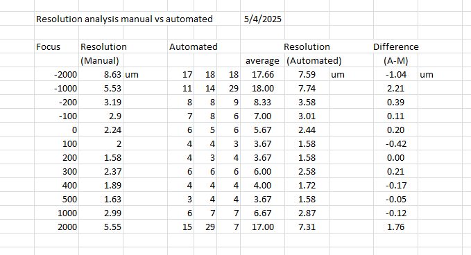
I ran a test where I imaged a sharp edge at various focus values after first doing an automated focus. I took those same images then ran your macro on the images, the results were very close, with the biggest difference at the most out of focus images. The images were all 0.43 um/pixel. At this point I really don’t understand your code, but very helpful and interesting. My plan is to run tests on 2 other scopes then possibly other methods like 2um beads. I am hoping to make some modifications to the scope to see if there are any changes in the resolution, but first I need a baseline. One possible way to improve the resolution would be to improve the lighting (I think). My long range goal is to measure images with super resolution modifications.
Expected resolution Resolution (r) = 0.61λ/NA = 0.61x520/0.22 = 1.44um
Thanks again for your help!
Awesome. This looks like an interesting project, feel free to post updates here if you have any.
Looks like there’s already a little room for improvement regarding the actual vs. theoretical optical resolution, based on your results. I’m sure a super resolution technique would make a large difference, if we’re not even at the optical resolution limit.
I did notice the test image you posted has JPEG artifacts, which would obviously mess things up. Was that originally a lossless image and the website perhaps just compressed it automatically?
The manual method I used involves doing 3 curve fits and looking for the intersections. Next finding the pixel length og the middle 10 to 90%. The variation I see is how to determine the fit of the dark and light regiond, expecially the dark region, it looks nonlinear.
The images I used were the max pixel depth I believe, 8MP, but it is a jpeg. I don’t know if a png or tiff file is available.
Got it. The method I did will probably yield different results, but I compute the full half width maximum FHWM of the line spread function (the derivative of the edge spread function). That’s probably at least partially why the manual vs. automatic estimates are different.
The Pi Camera can give a raw image. I think the OpenFlexure software does that, I don’t know what settings. I think that on a Pi the camera raw image is not as a different file format but uses metadata to put the actual raw image from the camera into the jpeg as metadata. You can tell because the jpegs become huge files, >20MB. Then you need to make that into a TIFF, or load the raw data into Python and do the demosaicing before processing the image.
Extracting the bayer data from the EXIF metadata is probably the best approach using the stock OFM software. I’ve never tried it, but I believe you just have to use the checkbox “Store Raw Data” and “Full Resolution”. It’s hard to say if it has been filtered in any way, since it passes through a proprietary driver: https://forums.raspberrypi.com/viewtopic.php?t=154915
If you’re willing to go through the extra work, you could write the code to capture the frames yourself and get the raw bayer data that way as well. Here’s an example:
from picamera2 import Picamera2
import numpy as np
from PIL import Image


def unpack(raw_bytes: np.ndarray):
    """
    Convert a 2D uint8 image with shape (H, W*2) to (H, W) 10-bit uint16 image.
    Each 2-byte pair encodes a 10-bit pixel.
    """
    h, w_bytes = raw_bytes.shape
    if w_bytes % 2 != 0:
        raise ValueError("Expected even number of bytes per row")

    w_pixels = w_bytes // 2
    # View as 16-bit little-endian
    raw_words = raw_bytes.reshape(h, w_pixels, 2)
    raw_10bit = (raw_words[:, :, 1].astype(np.uint16) <<
                 8) | raw_words[:, :, 0].astype(np.uint16)

    # If only 10 bits are valid, mask out the rest
    return raw_10bit & 0x03FF  # 10-bit mask


def main():
    picam2 = Picamera2()
    capture_config = picam2.create_still_configuration(
        raw={"format": 'SBGGR10'})
    picam2.configure(capture_config)
    picam2.start()
    print(picam2.stream_configuration("raw"))
    raw_data = picam2.capture_array("raw")
    data = unpack(raw_data)

    # This next line isn't really necessary, but helps when viewing the image
    # from a file explorer. When writing 16-bit PNGs, the full brightness is expected
    # to be at 65535. With 10-bit image data, the max is 1023. To avoid the images appearing
    # extremely dark, this line will scale the pixel intensity to 65535. However, the conversion
    # will cause rounding errors in the least significant bit. To be considered actual "raw" data,
    # this line should be removed. If the rounding errors in the LSB are acceptable, then this can
    # be a practical choice.
    data = (data.astype(np.uint32) * 65535 // 1023).astype(np.uint16)

    img = Image.fromarray(data, mode='I;16')
    img.save('bayer_preserved.png', format='PNG')


if __name__ == '__main__':
    main()
The raw bayer data gets saved (almost lossless) to a 16-bit PNG. You could make it lossless my taking out the scaling line that I commented. Here’s an example of the scaled version:

The image is in BW because I there’s no demosaicing - which I don’t believe is appropriate for what you’re doing. It also makes it very obvious that you actually get half the spatial resolution when you’re measuring the distance between green pixels.
Edit: Looks like this site does actually compress the images you upload. In my case, I uploaded a 3820x2464 16-bit PNG but it seems to have converted the sample image I provided to a 1920 × 1442 compressed JPEG. Here’s a download link to the original image: bayer_preserved.png - Google Drive
Edit 2: You can actually save it as a 16-bit PNG in a way that’s visible when opening it up in a regular viewer and without corrupting the data. If you left bit shift the raw 10-bit intensity by 6 instead of scaling it, you get a very clear image. If you want the original raw-10 bit data from the PNG, just right bit shift by 6. The reconstructed data using this method is always going to be equal to the original data, unlike if you were to scale it. Here’s what I mean:
def unpack(raw_bytes: np.ndarray):
    h, w_bytes = raw_bytes.shape
    if w_bytes % 2 != 0:
        raise ValueError('Width must be even (2 bytes per pixel).')

    w_pixels = w_bytes // 2
    raw_words = raw_bytes.reshape(h, w_pixels, 2)

    # Little-endian: byte[0] = LSB, byte[1] = MSB
    raw_10bit = (raw_words[:, :, 1].astype(
        np.uint16) << 8) | raw_words[:, :, 0]
    return (raw_10bit & 0x03FF) << 6

# and get rid of this line from the original script:
#   data = (data.astype(np.uint32) * 65535 // 1023).astype(np.uint16)
1 Like
You are a bit over my head, but I am very interested. For my manual analysis however I did convert the images to a grayscale, but not in ImageJ, I used IrfanVIEW, the image size dropped to (326KB) (8bit)
I think I saved the raw data, not sure yet. The original image is 12,639KB.
I opened up the original image and saved it with imageJ as a jpg (497KB)
I opened up the original image and saved it with ImageJ as a tiff (23,678KB)
I opened up the original image and saved it with ImageJ and saved it as an 8bit grayscale (457KB) - that’s different from IrfanVIEW?
I ran the python program on the images with the different pixel depths.
I used https://colab.research.google.com
There were some differences, but not very significant.In all cases the images were 3280 x 2464.

@DougKoebler it looks like your original JPEG is also compressed. For lossless RGB data, you’d get 3820x2464x3 bytes worth of data, which is about 27 MiB (or 28 MB). If you have raw bayer data, you’d have 3820x2464*2 bytes worth of data, which is about 18 MiB (or about 19 MB). Any time you’re using JPEG you’re going to have some form of compression, which will affect edges like the one you’re measuring. Any testing you do with a compressed image, no matter what programs you open with it afterwards, will be subject to the same loss.
Perhaps someone can post an example of how to capture and extract the bayer data using the OpenFlexure software, or link to an existing tutorial. Unfortunately my cat decided to knock my microscope off the shelf last night and broke the Z stage, so I can’t do anything with it until my new parts arrive in the mail.
I selected Full resolution, store raw data, took an image, then connected up to my PC and went to storage and opened up the image. Next I saved the image to my PC, (13,408KB)
I don’t see any other settings?
Theoretically, once you do get the raw data, it’s going to be in the form of metadata. So you’ll still have a JPEG, and you’ll still have lossly JPEG data, but there will be raw data in the EXIF section that you can extract. But you’re file size would be larger than what you’re getting, so it’s probably not working yet.
Looking at the code (openflexure_microscope/camera/pi.py · v2.11.0 · OpenFlexure / openflexure-microscope-server · GitLab), I wonder if there’s some sort of “video port” setting you can disable. It might be in the settings. If you don’t see something like that there, then I don’t really know why it’s not working. It’s too bad there isn’t an easier way, seems like a lot of hoops to jump through just to get raw data
@JohemianKnapsody do you know exactly what is stored for captures with the settings of @DougKoebler from post 17 above? Server v2.10.1 I believe.
Hi Taylor
I have a question. I tried to load your python script in Thonny on the Raspberry Pi.
I am trying to get that png image.
On the first line:
from picamera2 import Picamera2
ModuleNotFoundError: No module named ‘picamera2’
Am I in the correct place, using Thonny ?